Lesson Note on Linear Inequalities: Graphs and Applications for SSS 2

Class: Senior Secondary School 2 (SS2 / SSS 2)
Term: 2nd Term
Week: 9 – 10
Age: 16 years
Duration: 45 minutes
Subject: General Mathematics
Curriculum Theme: Algebra
Previous Lesson: .
Topic: LINEAR INEQUALITIES
Subject Matter: Linear inequalities in one variable, linear inequalities in two variables, range of values of combined inequalities, graph of linear inequalities in two variables, maximum and minimum values of simultaneous linear inequalities and application in real life situations

Specific Objectives

By the end of the lesson, pupils should be able to:

Cognitive Domain:

• Define linear inequalities and identify their symbols.
• Solve linear inequalities in one variable.
• Determine the range of values for combined linear inequalities.
• Identify the feasible region for simultaneous linear inequalities.

Affective Domain:

• Appreciate the importance of inequalities in various real-life situations.
• Show interest in solving mathematical problems involving inequalities.

Psychomotor Domain:

• Construct tables of values for linear inequalities in two variables.
• Draw graphs of linear inequalities in one and two variables on a number line and Cartesian plane.
• Locate maximum and minimum values from the feasible region of simultaneous inequalities.

Social Domain:

• Work collaboratively to solve inequality problems.
• Apply the concept of inequalities to solve everyday problems.

Reference Materials

The following resources were used in planning this lesson:

• 9 Years Basic Education Curriculum
• State Unified Scheme of Work
• New General Mathematics for Senior Secondary Schools 2
• https://www.mathsisfun.com/algebra/inequality-graphing.html
• https://www.khanacademy.org/math/algebra/x2f8bb11595b61c86:linear-inequalities-systems

Instructional Materials

The teacher will teach this lesson with the aid of:

• Scale balance
• Number line chart
• Graph board
• Mathematical sets

Rationale for the Lesson

This lesson helps pupils understand how to express and solve problems involving quantities that are not necessarily equal but have a range of possible values. It enables pupils to model real-world constraints and make informed decisions in various situations.

Prerequisite/Previous Knowledge

Pupils are expected to have prior knowledge of solving linear equations, basic algebraic operations, and representation of numbers on a number line.

Lesson Content/Board Summary

LINEAR INEQUALITIES

Meaning of Linear Inequalities

A linear inequality is a mathematical statement that compares two expressions using an inequality symbol. Unlike equations, which show equality, inequalities show a range of values. The common inequality symbols are:

• < (less than)
• > (greater than)
• ≤ (less than or equal to)
• ≥ (greater than or equal to)

Linear Inequalities in One Variable

These are inequalities involving a single variable, typically ‘x’, and can be represented on a number line. Solving linear inequalities in one variable is similar to solving linear equations, but with a key difference when multiplying or dividing by negative numbers.

Rules for Solving Linear Inequalities:

• Adding or subtracting the same number from both sides of an inequality does not change the direction of the inequality sign.
• Multiplying or dividing both sides by a positive number does not change the direction of the inequality sign.
• Multiplying or dividing both sides by a negative number reverses the direction of the inequality sign.

Example 1: Solve 3x – 5 < 7 and represent the solution on a number line.

Solution:
3x – 5 < 7
Step 1: Add 5 to both sides to isolate the term with x.
3x – 5 + 5 < 7 + 5
3x < 12
Step 2: Divide both sides by 3.
3x / 3 < 12 / 3
x < 4

Number Line Representation: An open circle at 4, with an arrow pointing to the left.

Example 2: Solve 10 – 2x ≥ 4 and represent the solution on a number line.

Solution:
10 – 2x ≥ 4
Step 1: Subtract 10 from both sides.
10 – 2x – 10 ≥ 4 – 10
-2x ≥ -6
Step 2: Divide both sides by -2. Remember to reverse the inequality sign.
-2x / -2 ≤ -6 / -2
x ≤ 3

Number Line Representation: A closed circle at 3, with an arrow pointing to the left.

Linear Inequalities in Two Variables

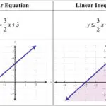
These inequalities involve two variables, usually ‘x’ and ‘y’, and are represented by a region on a Cartesian plane. The boundary line is drawn first, and then a test point is used to determine which region to shade.

Steps for Graphing Linear Inequalities in Two Variables:

1. Replace the inequality sign with an equality sign to get the equation of the boundary line.
2. Draw the boundary line:
   • Use a solid line for ≤ or ≥ (meaning points on the line are included in the solution).
   • Use a dotted or broken line for < or > (meaning points on the line are not included).
3. Choose a test point not on the line (e.g., (0,0) if the line does not pass through the origin).
4. Substitute the coordinates of the test point into the original inequality.
5. If the inequality is true, shade the region containing the test point. If false, shade the opposite region.

Example: Graph the inequality y > 2x – 1.

Solution:
Step 1: Draw the line y = 2x – 1.
When x = 0, y = -1. (0, -1)
When y = 0, 0 = 2x – 1 => 2x = 1 => x = 0.5. (0.5, 0)
Step 2: Draw a dotted line through (0, -1) and (0.5, 0) because the inequality is >.
Step 3: Test a point, e.g., (0,0).
Substitute (0,0) into y > 2x – 1:
0 > 2(0) – 1
0 > -1 (This is true).
Step 4: Shade the region that contains the point (0,0).

Range of Values of Combined Inequalities

Combined inequalities involve two or more inequalities joined together. To solve them, each part is solved independently, and then the solutions are combined to find the common range of values that satisfy all inequalities. This can be represented on a single number line.

Example: Solve -3 ≤ 2x + 1 < 7.

Solution:
This can be split into two separate inequalities:
1) -3 ≤ 2x + 1
2) 2x + 1 < 7

Solve 1):
-3 ≤ 2x + 1
-3 – 1 ≤ 2x
-4 ≤ 2x
-4 / 2 ≤ 2x / 2
-2 ≤ x (or x ≥ -2)

Solve 2):
2x + 1 < 7
2x < 7 – 1
2x < 6
2x / 2 < 6 / 2
x < 3

Combine the solutions: x ≥ -2 and x < 3.
This means -2 ≤ x < 3.

Number Line Representation: A closed circle at -2 and an open circle at 3, with the line segment between them shaded.

Maximum and Minimum Values of Simultaneous Linear Inequalities and Application in Real Life Situations

When multiple linear inequalities are considered together, they form a system of linear inequalities. The solution set for such a system is the region on the graph that satisfies all inequalities simultaneously. This region is called the feasible region.

Finding Maximum and Minimum Values:

In linear programming, we often need to find the maximum or minimum value of an objective function (e.g., profit, cost) subject to certain constraints (given as linear inequalities). The maximum or minimum values usually occur at the vertices (corner points) of the feasible region.

Steps:

1. Graph all the inequalities on the same Cartesian plane.
2. Identify the feasible region (the area where all shaded regions overlap).
3. Determine the coordinates of the vertices (corner points) of the feasible region. These points are found by solving the equations of the lines that intersect at each vertex.
4. If an objective function (e.g., P = ax + by) is given, substitute the coordinates of each vertex into the objective function to find the corresponding value.
5. The largest value will be the maximum, and the smallest will be the minimum.

Example: Find the vertices of the feasible region defined by the inequalities: x ≥ 0, y ≥ 0, x + y ≤ 5.

Solution:
Step 1: Graph the boundary lines:
x = 0 (y-axis)
y = 0 (x-axis)
x + y = 5 (line passing through (5,0) and (0,5))
Step 2: Identify the feasible region.
x ≥ 0 means the region to the right of the y-axis.
y ≥ 0 means the region above the x-axis.
x + y ≤ 5 means the region below the line x + y = 5 (test (0,0): 0+0 ≤ 5 is true).
The feasible region is the triangle formed by the origin and the intercepts of x + y = 5.
Step 3: Determine the vertices.
The vertices are the points where the boundary lines intersect:
Intersection of x = 0 and y = 0 is (0,0).
Intersection of y = 0 and x + y = 5 is (5,0).
Intersection of x = 0 and x + y = 5 is (0,5).
The vertices of the feasible region are (0,0), (5,0), and (0,5).

Real-Life Applications of Linear Inequalities:

Linear inequalities are used in many practical situations, including:

• Budgeting: Determining how much money can be spent on different items without exceeding a total budget.
• Resource Allocation: Deciding how to distribute limited resources (e.g., time, materials, labor) to maximize output or minimize cost.
• Production Planning: Managing production levels to meet demand while staying within capacity limits.
• Nutrition: Planning diets to ensure minimum nutrient intake without exceeding calorie limits.
• Manufacturing: Ensuring product specifications meet certain tolerances (e.g., a component must be between 10mm and 10.5mm).

Teaching Methods/Instructional Techniques

Discussion, Lecture, Demonstration, Question and Answer, Visual Aids

Instructional Procedures

Step 1: Introduction

Time: 5 minutes
Teaching Skill: Set Induction
Teacher’s Activity: The teacher introduces the lesson by using a scale balance to demonstrate the concept of inequality. The teacher places unequal weights on the balance to show one side being heavier or lighter than the other, then relates this to mathematical inequality symbols. The teacher also asks pupils to recall what an equation is and how it differs from an inequality.
Pupils’ Activity: Pupils observe the demonstration and respond to the teacher’s questions, recalling their knowledge of equations and making observations about the scale balance.
Learning Point: Pupils are introduced to the concept of inequality and its real-world representation, linking it to mathematics.

Step 2: Linear Inequalities in One Variable

Time: 10 minutes
Teaching Skill: Explanation/Demonstration
Teacher’s Activity: The teacher defines linear inequalities and explains the four inequality symbols. The teacher then guides pupils through the rules for solving linear inequalities in one variable, paying special attention to reversing the inequality sign when multiplying or dividing by a negative number. The teacher solves examples on the board, demonstrating how to represent solutions on a number line.
Pupils’ Activity: Pupils listen attentively, take notes, and ask questions for clarification. They participate in solving example problems on the board and practice representing solutions on number lines.
Learning Point: Pupils learn how to solve and graphically represent linear inequalities in one variable.

Step 3: Linear Inequalities in Two Variables

Time: 10 minutes
Teaching Skill: Explanation/Demonstration
Teacher’s Activity: The teacher explains how linear inequalities in two variables differ from those in one variable. The teacher demonstrates the steps for graphing linear inequalities in two variables on a Cartesian plane, including drawing solid/dotted lines and shading the correct region using a test point. The teacher provides examples and guides pupils through the process.
Pupils’ Activity: Pupils observe the teacher’s demonstration on the graph board, ask questions about the steps, and attempt to draw simple graphs in their notebooks.
Learning Point: Pupils understand how to graph linear inequalities involving two variables.

Step 4: Range of Values of Combined Inequalities

Time: 5 minutes
Teaching Skill: Explanation/Guided Practice
Teacher’s Activity: The teacher explains how to solve combined linear inequalities by splitting them into two separate inequalities, solving each, and then combining the solutions to find the common range of values. The teacher shows how to represent the combined solution on a single number line.
Pupils’ Activity: Pupils follow the teacher’s explanation and work through an example, practicing how to combine solutions and represent them graphically.
Learning Point: Pupils learn to solve and represent combined linear inequalities.

Step 5: Maximum and Minimum Values of Simultaneous Linear Inequalities

Time: 5 minutes
Teaching Skill: Explanation/Illustrative
Teacher’s Activity: The teacher introduces the concept of simultaneous linear inequalities and the feasible region. The teacher explains that maximum and minimum values of an objective function occur at the vertices of this feasible region. The teacher illustrates with a simple example, showing how to identify the feasible region and its corner points.
Pupils’ Activity: Pupils listen and try to grasp the concept of the feasible region and its vertices. They observe how corner points are determined from the graph.
Learning Point: Pupils understand the concept of a feasible region and how it relates to finding maximum and minimum values.

Step 6: Application in Real Life Situations

Time: 5 minutes
Teaching Skill: Discussion/Application
Teacher’s Activity: The teacher leads a brief discussion on various real-life scenarios where linear inequalities are used, such as budgeting, resource allocation, and production planning. The teacher encourages pupils to think of other examples.
Pupils’ Activity: Pupils contribute examples of real-life situations where inequalities might be applied and discuss their relevance.
Learning Point: Pupils connect the mathematical concept of inequalities to practical, everyday problems.

Step 7: Evaluation/Review

Time: 5 minutes

Teaching Skill: Questioning/Assessment

Teacher’s Activity: The teacher evaluates the learning by asking the following questions:

1. Define a linear inequality.
2. State the four common inequality symbols.
3. Solve the inequality: 2x + 3 > 9.
4. Explain when you should reverse the inequality sign while solving.
5. Mention two real-life applications of linear inequalities.

Pupils’ Activity: Pupils answer orally and in writing.

Learning Point: Pupils demonstrate understanding of the lesson.

Step 8: Conclusion

Time: 5 minutes
Teaching Skill: Summarization/Assignment
Teacher’s Activity: The teacher summarizes the key points of the lesson, reinforcing the understanding of solving and graphing linear inequalities in one and two variables, combined inequalities, and their real-life applications. The teacher gives homework problems for practice.
Pupils’ Activity: Pupils listen to the summary, ask any remaining questions, and copy down the homework assignment.
Learning Point: Pupils consolidate their learning and prepare for independent practice.

Lesson Keywords

• Inequality – A mathematical statement comparing two expressions that are not equal, using symbols like <, >, ≤, or ≥.
• Linear Inequality – An inequality where the highest power of the variable(s) is one.
• Number Line – A visual representation of numbers as points on a straight line.
• Cartesian Plane – A two-dimensional plane used to graph points and functions, defined by perpendicular x and y axes.
• Feasible Region – The region on a graph that satisfies all conditions (inequalities) of a system.
• Vertices – The corner points of the feasible region, where boundary lines intersect.

Differentiation

For pupils who grasp the concepts quickly, the teacher will provide more complex problems involving multiple inequalities and real-world word problems to challenge them. For pupils who require additional support, the teacher will provide simplified examples, offer one-on-one guidance, and use more visual aids like pre-drawn graphs to illustrate concepts.

Note for teachers using this lesson plan

Ensure a strong foundation in solving linear equations before introducing inequalities. Emphasize the rule of reversing the inequality sign when multiplying or dividing by a negative number, as this is a common area of error. Encourage pupils to use graph paper for two-variable inequalities to ensure accuracy. Practical examples should be used to make the lesson relatable and engaging for pupils.